This is an R script ported from here.
# Load packages
library("dplyr")
library("ggplot2")
library("nycflights13")
library("lubridate")
# it's a data.frame, but also a tbl_df.
# doesn't print entire thing to screen.
flights## # A tibble: 336,776 x 19
## year month day dep_time sched_dep_time dep_delay arr_time
## <int> <int> <int> <int> <int> <dbl> <int>
## 1 2013 1 1 517 515 2 830
## 2 2013 1 1 533 529 4 850
## 3 2013 1 1 542 540 2 923
## 4 2013 1 1 544 545 -1 1004
## 5 2013 1 1 554 600 -6 812
## 6 2013 1 1 554 558 -4 740
## 7 2013 1 1 555 600 -5 913
## 8 2013 1 1 557 600 -3 709
## 9 2013 1 1 557 600 -3 838
## 10 2013 1 1 558 600 -2 753
## # ... with 336,766 more rows, and 12 more variables: sched_arr_time <int>,
## # arr_delay <dbl>, carrier <chr>, flight <int>, tailnum <chr>,
## # origin <chr>, dest <chr>, air_time <dbl>, distance <dbl>, hour <dbl>,
## # minute <dbl>, time_hour <dttm>class(flights)## [1] "tbl_df" "tbl" "data.frame"weather## # A tibble: 26,130 x 15
## origin year month day hour temp dewp humid wind_dir wind_speed
## <chr> <dbl> <dbl> <int> <int> <dbl> <dbl> <dbl> <dbl> <dbl>
## 1 EWR 2013 1 1 0 37.04 21.92 53.97 230 10.35702
## 2 EWR 2013 1 1 1 37.04 21.92 53.97 230 13.80936
## 3 EWR 2013 1 1 2 37.94 21.92 52.09 230 12.65858
## 4 EWR 2013 1 1 3 37.94 23.00 54.51 230 13.80936
## 5 EWR 2013 1 1 4 37.94 24.08 57.04 240 14.96014
## 6 EWR 2013 1 1 6 39.02 26.06 59.37 270 10.35702
## 7 EWR 2013 1 1 7 39.02 26.96 61.63 250 8.05546
## 8 EWR 2013 1 1 8 39.02 28.04 64.43 240 11.50780
## 9 EWR 2013 1 1 9 39.92 28.04 62.21 250 12.65858
## 10 EWR 2013 1 1 10 39.02 28.04 64.43 260 12.65858
## # ... with 26,120 more rows, and 5 more variables: wind_gust <dbl>,
## # precip <dbl>, pressure <dbl>, visib <dbl>, time_hour <dttm>planes## # A tibble: 3,322 x 9
## tailnum year type manufacturer model
## <chr> <int> <chr> <chr> <chr>
## 1 N10156 2004 Fixed wing multi engine EMBRAER EMB-145XR
## 2 N102UW 1998 Fixed wing multi engine AIRBUS INDUSTRIE A320-214
## 3 N103US 1999 Fixed wing multi engine AIRBUS INDUSTRIE A320-214
## 4 N104UW 1999 Fixed wing multi engine AIRBUS INDUSTRIE A320-214
## 5 N10575 2002 Fixed wing multi engine EMBRAER EMB-145LR
## 6 N105UW 1999 Fixed wing multi engine AIRBUS INDUSTRIE A320-214
## 7 N107US 1999 Fixed wing multi engine AIRBUS INDUSTRIE A320-214
## 8 N108UW 1999 Fixed wing multi engine AIRBUS INDUSTRIE A320-214
## 9 N109UW 1999 Fixed wing multi engine AIRBUS INDUSTRIE A320-214
## 10 N110UW 1999 Fixed wing multi engine AIRBUS INDUSTRIE A320-214
## # ... with 3,312 more rows, and 4 more variables: engines <int>,
## # seats <int>, speed <int>, engine <chr>airports## # A tibble: 1,458 x 8
## faa name lat lon alt tz
## <chr> <chr> <dbl> <dbl> <int> <dbl>
## 1 04G Lansdowne Airport 41.13047 -80.61958 1044 -5
## 2 06A Moton Field Municipal Airport 32.46057 -85.68003 264 -6
## 3 06C Schaumburg Regional 41.98934 -88.10124 801 -6
## 4 06N Randall Airport 41.43191 -74.39156 523 -5
## 5 09J Jekyll Island Airport 31.07447 -81.42778 11 -5
## 6 0A9 Elizabethton Municipal Airport 36.37122 -82.17342 1593 -5
## 7 0G6 Williams County Airport 41.46731 -84.50678 730 -5
## 8 0G7 Finger Lakes Regional Airport 42.88356 -76.78123 492 -5
## 9 0P2 Shoestring Aviation Airfield 39.79482 -76.64719 1000 -5
## 10 0S9 Jefferson County Intl 48.05381 -122.81064 108 -8
## # ... with 1,448 more rows, and 2 more variables: dst <chr>, tzone <chr>airlines## # A tibble: 16 x 2
## carrier name
## <chr> <chr>
## 1 9E Endeavor Air Inc.
## 2 AA American Airlines Inc.
## 3 AS Alaska Airlines Inc.
## 4 B6 JetBlue Airways
## 5 DL Delta Air Lines Inc.
## 6 EV ExpressJet Airlines Inc.
## 7 F9 Frontier Airlines Inc.
## 8 FL AirTran Airways Corporation
## 9 HA Hawaiian Airlines Inc.
## 10 MQ Envoy Air
## 11 OO SkyWest Airlines Inc.
## 12 UA United Air Lines Inc.
## 13 US US Airways Inc.
## 14 VX Virgin America
## 15 WN Southwest Airlines Co.
## 16 YV Mesa Airlines Inc.# dplyr also gives you verbs. All take a tbl_df as first argument.
# on their own, not much that base R can't do.
## select particular variables from flights
select(flights, year, month, day)## # A tibble: 336,776 x 3
## year month day
## <int> <int> <int>
## 1 2013 1 1
## 2 2013 1 1
## 3 2013 1 1
## 4 2013 1 1
## 5 2013 1 1
## 6 2013 1 1
## 7 2013 1 1
## 8 2013 1 1
## 9 2013 1 1
## 10 2013 1 1
## # ... with 336,766 more rows## filter based on some condition. all fights taken by this plane.
filter(flights, tailnum=="N14228")## # A tibble: 111 x 19
## year month day dep_time sched_dep_time dep_delay arr_time
## <int> <int> <int> <int> <int> <dbl> <int>
## 1 2013 1 1 517 515 2 830
## 2 2013 1 8 1435 1440 -5 1717
## 3 2013 1 9 717 700 17 812
## 4 2013 1 9 1143 1144 -1 1425
## 5 2013 1 13 835 824 11 1030
## 6 2013 1 16 1829 1730 59 2117
## 7 2013 1 22 1902 1808 54 2214
## 8 2013 1 23 1050 1056 -6 1143
## 9 2013 1 23 1533 1529 4 1641
## 10 2013 1 25 724 720 4 1000
## # ... with 101 more rows, and 12 more variables: sched_arr_time <int>,
## # arr_delay <dbl>, carrier <chr>, flight <int>, tailnum <chr>,
## # origin <chr>, dest <chr>, air_time <dbl>, distance <dbl>, hour <dbl>,
## # minute <dbl>, time_hour <dttm>## mutate adds new columns. time made up in air:
mutate(flights, madeup=dep_delay-arr_delay)## # A tibble: 336,776 x 20
## year month day dep_time sched_dep_time dep_delay arr_time
## <int> <int> <int> <int> <int> <dbl> <int>
## 1 2013 1 1 517 515 2 830
## 2 2013 1 1 533 529 4 850
## 3 2013 1 1 542 540 2 923
## 4 2013 1 1 544 545 -1 1004
## 5 2013 1 1 554 600 -6 812
## 6 2013 1 1 554 558 -4 740
## 7 2013 1 1 555 600 -5 913
## 8 2013 1 1 557 600 -3 709
## 9 2013 1 1 557 600 -3 838
## 10 2013 1 1 558 600 -2 753
## # ... with 336,766 more rows, and 13 more variables: sched_arr_time <int>,
## # arr_delay <dbl>, carrier <chr>, flight <int>, tailnum <chr>,
## # origin <chr>, dest <chr>, air_time <dbl>, distance <dbl>, hour <dbl>,
## # minute <dbl>, time_hour <dttm>, madeup <dbl>## summarize reduces grouped data to a single row.
summarize(flights, avgdelay=mean(arr_delay, na.rm=TRUE))## # A tibble: 1 x 1
## avgdelay
## <dbl>
## 1 6.895377## group_by turns existing table into grouped_df class
## summary operations are performed by the group
group_by(flights, dest)## # A tibble: 336,776 x 19
## # Groups: dest [105]
## year month day dep_time sched_dep_time dep_delay arr_time
## <int> <int> <int> <int> <int> <dbl> <int>
## 1 2013 1 1 517 515 2 830
## 2 2013 1 1 533 529 4 850
## 3 2013 1 1 542 540 2 923
## 4 2013 1 1 544 545 -1 1004
## 5 2013 1 1 554 600 -6 812
## 6 2013 1 1 554 558 -4 740
## 7 2013 1 1 555 600 -5 913
## 8 2013 1 1 557 600 -3 709
## 9 2013 1 1 557 600 -3 838
## 10 2013 1 1 558 600 -2 753
## # ... with 336,766 more rows, and 12 more variables: sched_arr_time <int>,
## # arr_delay <dbl>, carrier <chr>, flight <int>, tailnum <chr>,
## # origin <chr>, dest <chr>, air_time <dbl>, distance <dbl>, hour <dbl>,
## # minute <dbl>, time_hour <dttm>summarize(group_by(flights, dest), avgdelay=mean(arr_delay, na.rm=TRUE))## # A tibble: 105 x 2
## dest avgdelay
## <chr> <dbl>
## 1 ABQ 4.381890
## 2 ACK 4.852273
## 3 ALB 14.397129
## 4 ANC -2.500000
## 5 ATL 11.300113
## 6 AUS 6.019909
## 7 AVL 8.003831
## 8 BDL 7.048544
## 9 BGR 8.027933
## 10 BHM 16.877323
## # ... with 95 more rows# Combining
# 1. flights dataset
# 2. mutate to add "madeup" variable
# 3. filter it where madeup>60
# 4. select particular columns
# %>% as "then"
select(
filter(
mutate(flights,
madeup=dep_delay-arr_delay
), madeup>60
), dep_delay, arr_delay, dest, madeup
)## # A tibble: 154 x 4
## dep_delay arr_delay dest madeup
## <dbl> <dbl> <chr> <dbl>
## 1 -4 -65 LAX 61
## 2 65 1 OAK 64
## 3 12 -57 SFO 69
## 4 -4 -70 SFO 66
## 5 121 57 LAX 64
## 6 9 -63 LAX 72
## 7 46 -16 LAX 62
## 8 37 -25 SFO 62
## 9 -3 -68 LAS 65
## 10 31 -42 SFO 73
## # ... with 144 more rowsflights## # A tibble: 336,776 x 19
## year month day dep_time sched_dep_time dep_delay arr_time
## <int> <int> <int> <int> <int> <dbl> <int>
## 1 2013 1 1 517 515 2 830
## 2 2013 1 1 533 529 4 850
## 3 2013 1 1 542 540 2 923
## 4 2013 1 1 544 545 -1 1004
## 5 2013 1 1 554 600 -6 812
## 6 2013 1 1 554 558 -4 740
## 7 2013 1 1 555 600 -5 913
## 8 2013 1 1 557 600 -3 709
## 9 2013 1 1 557 600 -3 838
## 10 2013 1 1 558 600 -2 753
## # ... with 336,766 more rows, and 12 more variables: sched_arr_time <int>,
## # arr_delay <dbl>, carrier <chr>, flight <int>, tailnum <chr>,
## # origin <chr>, dest <chr>, air_time <dbl>, distance <dbl>, hour <dbl>,
## # minute <dbl>, time_hour <dttm>flights %>%
mutate(madeup=dep_delay-arr_delay) %>%
filter(madeup>60) %>%
select(dep_delay, arr_delay, dest, madeup)## # A tibble: 154 x 4
## dep_delay arr_delay dest madeup
## <dbl> <dbl> <chr> <dbl>
## 1 -4 -65 LAX 61
## 2 65 1 OAK 64
## 3 12 -57 SFO 69
## 4 -4 -70 SFO 66
## 5 121 57 LAX 64
## 6 9 -63 LAX 72
## 7 46 -16 LAX 62
## 8 37 -25 SFO 62
## 9 -3 -68 LAS 65
## 10 31 -42 SFO 73
## # ... with 144 more rows# add a date to flights
flights## # A tibble: 336,776 x 19
## year month day dep_time sched_dep_time dep_delay arr_time
## <int> <int> <int> <int> <int> <dbl> <int>
## 1 2013 1 1 517 515 2 830
## 2 2013 1 1 533 529 4 850
## 3 2013 1 1 542 540 2 923
## 4 2013 1 1 544 545 -1 1004
## 5 2013 1 1 554 600 -6 812
## 6 2013 1 1 554 558 -4 740
## 7 2013 1 1 555 600 -5 913
## 8 2013 1 1 557 600 -3 709
## 9 2013 1 1 557 600 -3 838
## 10 2013 1 1 558 600 -2 753
## # ... with 336,766 more rows, and 12 more variables: sched_arr_time <int>,
## # arr_delay <dbl>, carrier <chr>, flight <int>, tailnum <chr>,
## # origin <chr>, dest <chr>, air_time <dbl>, distance <dbl>, hour <dbl>,
## # minute <dbl>, time_hour <dttm>flights <- flights %>%
mutate(date=ymd(paste(year, month, day, sep="-"))) %>%
na.omit()
flights## # A tibble: 327,346 x 20
## year month day dep_time sched_dep_time dep_delay arr_time
## <int> <int> <int> <int> <int> <dbl> <int>
## 1 2013 1 1 517 515 2 830
## 2 2013 1 1 533 529 4 850
## 3 2013 1 1 542 540 2 923
## 4 2013 1 1 544 545 -1 1004
## 5 2013 1 1 554 600 -6 812
## 6 2013 1 1 554 558 -4 740
## 7 2013 1 1 555 600 -5 913
## 8 2013 1 1 557 600 -3 709
## 9 2013 1 1 557 600 -3 838
## 10 2013 1 1 558 600 -2 753
## # ... with 327,336 more rows, and 13 more variables: sched_arr_time <int>,
## # arr_delay <dbl>, carrier <chr>, flight <int>, tailnum <chr>,
## # origin <chr>, dest <chr>, air_time <dbl>, distance <dbl>, hour <dbl>,
## # minute <dbl>, time_hour <dttm>, date <date>flights %>% select(date)## # A tibble: 327,346 x 1
## date
## <date>
## 1 2013-01-01
## 2 2013-01-01
## 3 2013-01-01
## 4 2013-01-01
## 5 2013-01-01
## 6 2013-01-01
## 7 2013-01-01
## 8 2013-01-01
## 9 2013-01-01
## 10 2013-01-01
## # ... with 327,336 more rowsclass(flights$date)## [1] "Date"# How many flights departed each day?
flights %>% group_by(date) %>% summarize(n=n())## # A tibble: 365 x 2
## date n
## <date> <int>
## 1 2013-01-01 831
## 2 2013-01-02 928
## 3 2013-01-03 900
## 4 2013-01-04 908
## 5 2013-01-05 717
## 6 2013-01-06 829
## 7 2013-01-07 930
## 8 2013-01-08 892
## 9 2013-01-09 893
## 10 2013-01-10 929
## # ... with 355 more rows# How many each day from each origin?
flights %>% group_by(date, origin) %>% summarize(n=n())## # A tibble: 1,095 x 3
## # Groups: date [?]
## date origin n
## <date> <chr> <int>
## 1 2013-01-01 EWR 300
## 2 2013-01-01 JFK 295
## 3 2013-01-01 LGA 236
## 4 2013-01-02 EWR 341
## 5 2013-01-02 JFK 317
## 6 2013-01-02 LGA 270
## 7 2013-01-03 EWR 331
## 8 2013-01-03 JFK 317
## 9 2013-01-03 LGA 252
## 10 2013-01-04 EWR 337
## # ... with 1,085 more rows# how many by week by origin?
flights %>% group_by(week(date), origin) %>% summarize(n=n())## # A tibble: 159 x 3
## # Groups: week(date) [?]
## `week(date)` origin n
## <dbl> <chr> <int>
## 1 1 EWR 2187
## 2 1 JFK 2157
## 3 1 LGA 1699
## 4 2 EWR 2208
## 5 2 JFK 2043
## 6 2 LGA 1791
## 7 3 EWR 2170
## 8 3 JFK 1997
## 9 3 LGA 1746
## 10 4 EWR 2129
## # ... with 149 more rows# we can name a variable in the resulting tbl_df
flights %>% group_by(week=week(date), origin) %>% summarize(n=n())## # A tibble: 159 x 3
## # Groups: week [?]
## week origin n
## <dbl> <chr> <int>
## 1 1 EWR 2187
## 2 1 JFK 2157
## 3 1 LGA 1699
## 4 2 EWR 2208
## 5 2 JFK 2043
## 6 2 LGA 1791
## 7 3 EWR 2170
## 8 3 JFK 1997
## 9 3 LGA 1746
## 10 4 EWR 2129
## # ... with 149 more rows# let's create new data grouped by week and destination
# showing number of flights, average delays, and number distinct destinations
byweek <- flights %>%
group_by(week=week(date), origin) %>%
summarize(n=n(), delay=mean(arr_delay), ndests=n_distinct(dest))
byweek## # A tibble: 159 x 5
## # Groups: week [?]
## week origin n delay ndests
## <dbl> <chr> <int> <dbl> <int>
## 1 1 EWR 2187 9.0740741 82
## 2 1 JFK 2157 0.2814094 60
## 3 1 LGA 1699 1.8022366 44
## 4 2 EWR 2208 3.1077899 80
## 5 2 JFK 2043 -2.2623593 59
## 6 2 LGA 1791 -4.8330542 40
## 7 3 EWR 2170 15.0589862 80
## 8 3 JFK 1997 -1.5578368 58
## 9 3 LGA 1746 6.0337915 39
## 10 4 EWR 2129 18.7745420 80
## # ... with 149 more rows# plot number of flights by week by origin city
byweek %>% ggplot(aes(week, n, colour=origin)) + geom_line()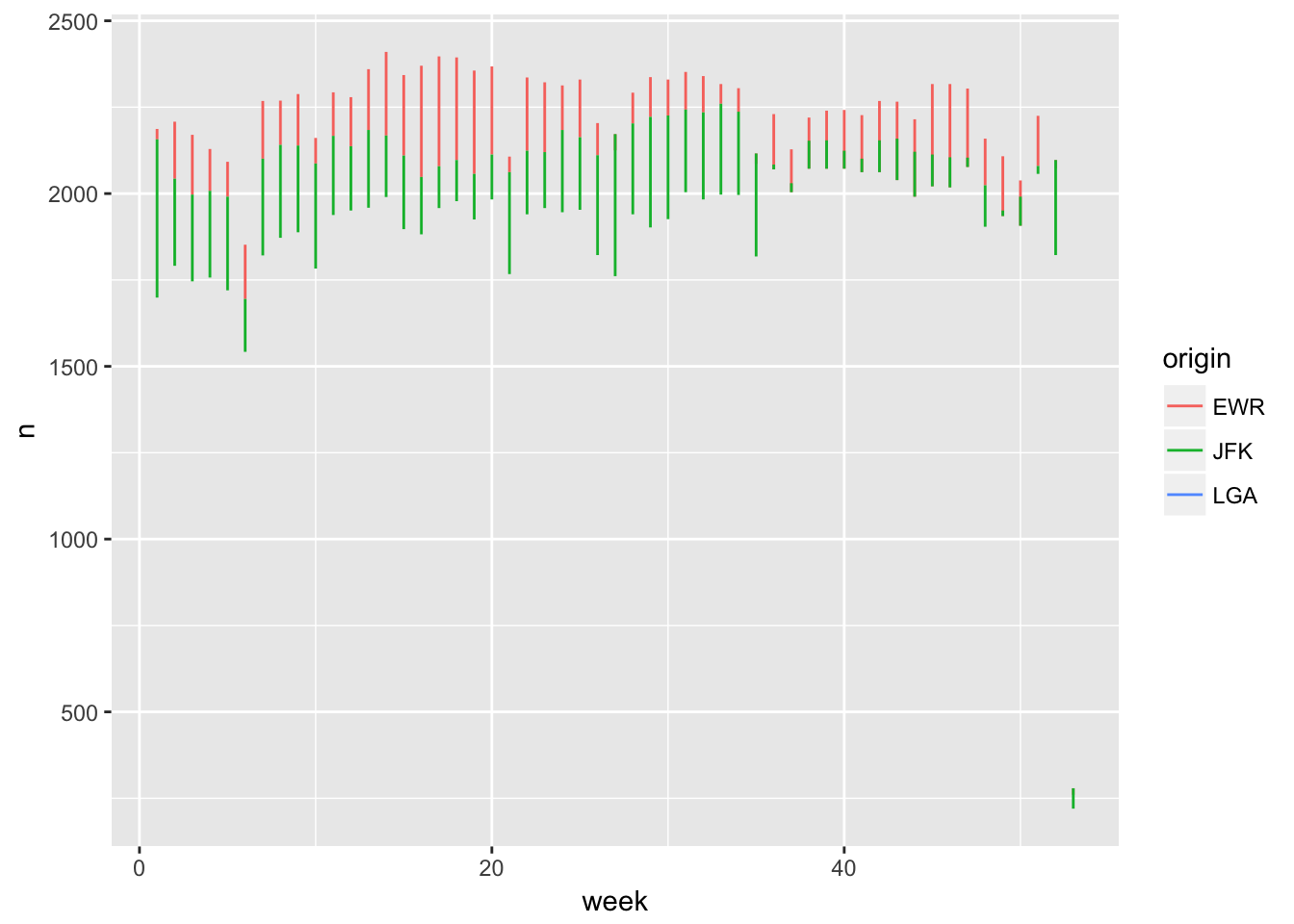
# why the dip at the end?
# let's get total number of flights by week
byweek %>% summarize(sum(n))
## # A tibble: 53 x 2
## week `sum(n)`
## <dbl> <int>
## 1 1 6043
## 2 2 6042
## 3 3 5913
## 4 4 5894
## 5 5 5803
## 6 6 5089
## 7 7 6190
## 8 8 6282
## 9 9 6315
## 10 10 6031
## # ... with 43 more rows# only 364 days in year, Dec 31 is probably day 1 of week 53
52*7## [1] 364# same plot but not looking at week 53
byweek %>%
filter(week<=52) %>%
ggplot(aes(week, n, colour=origin)) + geom_line()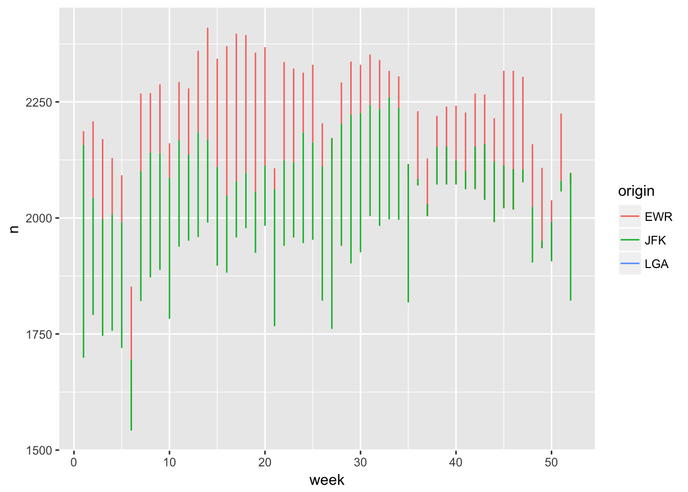
ymd("2013-01-01") + weeks(21) # mem day## [1] "2013-05-28"ymd("2013-01-01") + weeks(26) # july 4## [1] "2013-07-02"ymd("2013-01-01") + weeks(35) # labor day. why JFK continues decline?## [1] "2013-09-03"ymd("2013-01-01") + weeks(47) # TG, xmas, NY## [1] "2013-11-26"# why JFK lose number after labor day?
# LGA added a LOT more destinations just before this decline.
# makes more people fly out of there as opposed to JFK!
byweek %>%
filter(week<=52) %>%
ggplot(aes(week, ndests, colour=origin)) + geom_line()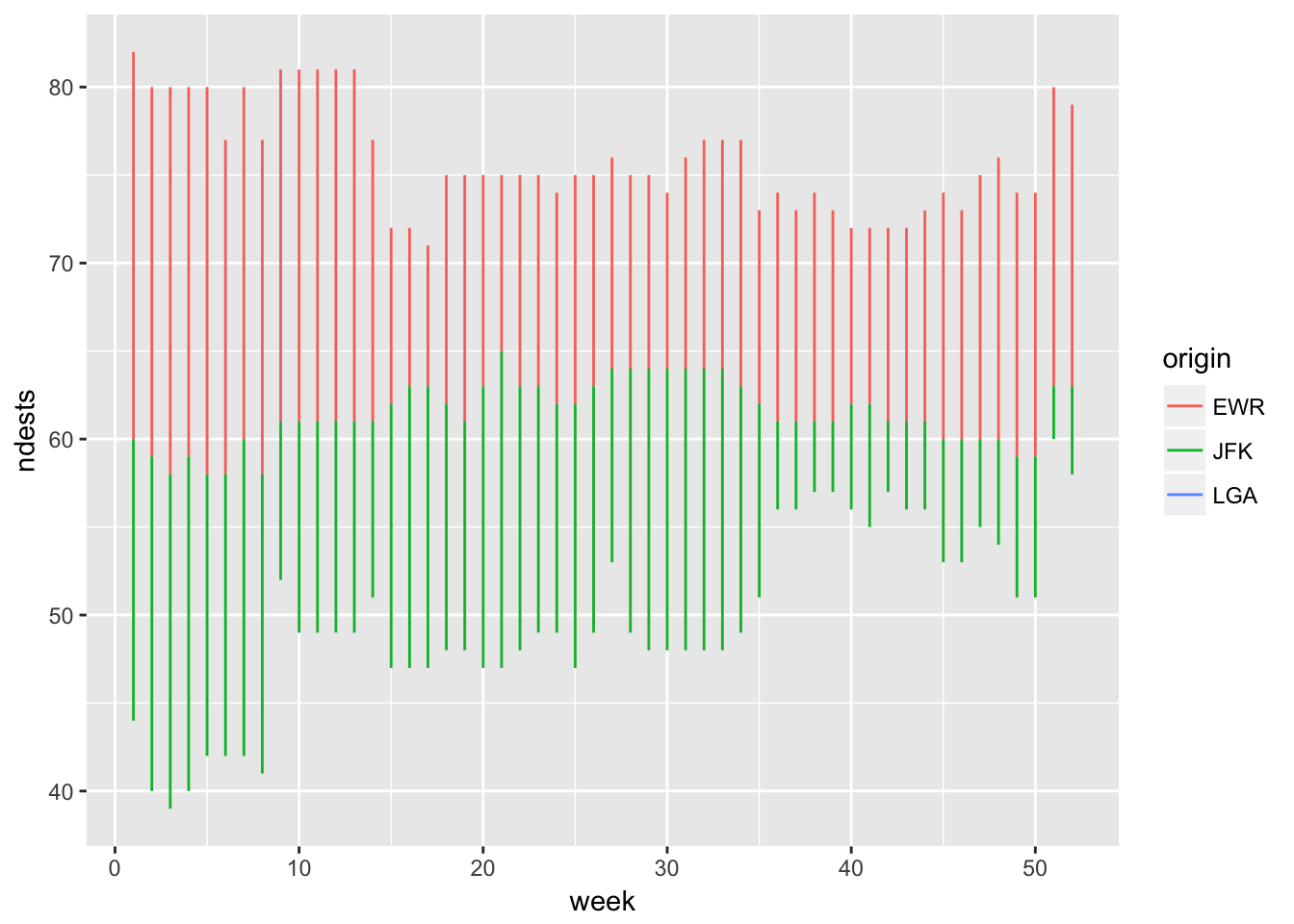
# What causes delays?
# do older planes have more delays?
flights
## # A tibble: 327,346 x 20
## year month day dep_time sched_dep_time dep_delay arr_time
## <int> <int> <int> <int> <int> <dbl> <int>
## 1 2013 1 1 517 515 2 830
## 2 2013 1 1 533 529 4 850
## 3 2013 1 1 542 540 2 923
## 4 2013 1 1 544 545 -1 1004
## 5 2013 1 1 554 600 -6 812
## 6 2013 1 1 554 558 -4 740
## 7 2013 1 1 555 600 -5 913
## 8 2013 1 1 557 600 -3 709
## 9 2013 1 1 557 600 -3 838
## 10 2013 1 1 558 600 -2 753
## # ... with 327,336 more rows, and 13 more variables: sched_arr_time <int>,
## # arr_delay <dbl>, carrier <chr>, flight <int>, tailnum <chr>,
## # origin <chr>, dest <chr>, air_time <dbl>, distance <dbl>, hour <dbl>,
## # minute <dbl>, time_hour <dttm>, date <date>planes## # A tibble: 3,322 x 9
## tailnum year type manufacturer model
## <chr> <int> <chr> <chr> <chr>
## 1 N10156 2004 Fixed wing multi engine EMBRAER EMB-145XR
## 2 N102UW 1998 Fixed wing multi engine AIRBUS INDUSTRIE A320-214
## 3 N103US 1999 Fixed wing multi engine AIRBUS INDUSTRIE A320-214
## 4 N104UW 1999 Fixed wing multi engine AIRBUS INDUSTRIE A320-214
## 5 N10575 2002 Fixed wing multi engine EMBRAER EMB-145LR
## 6 N105UW 1999 Fixed wing multi engine AIRBUS INDUSTRIE A320-214
## 7 N107US 1999 Fixed wing multi engine AIRBUS INDUSTRIE A320-214
## 8 N108UW 1999 Fixed wing multi engine AIRBUS INDUSTRIE A320-214
## 9 N109UW 1999 Fixed wing multi engine AIRBUS INDUSTRIE A320-214
## 10 N110UW 1999 Fixed wing multi engine AIRBUS INDUSTRIE A320-214
## # ... with 3,312 more rows, and 4 more variables: engines <int>,
## # seats <int>, speed <int>, engine <chr>flights %>%
inner_join(planes, by="tailnum") %>% # explain year.x, .y
group_by(year.y) %>%
summarize(delay=mean(arr_delay)) %>%
filter(!is.na(year.y)) %>%
ggplot(aes(year.y, delay)) + geom_point() + geom_smooth(method="loess")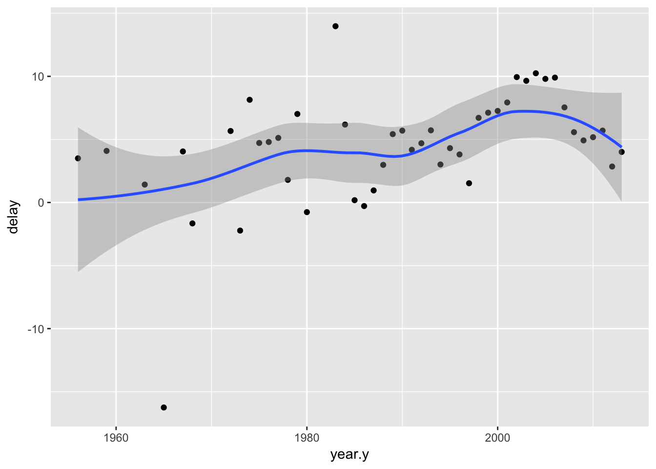
# what about weather?
# look at delays by month by destination
flights %>%
  group_by(month, origin) %>%
  summarize(delay=mean(arr_delay)) %>%
  ggplot(aes(month, delay, fill=origin)) + geom_bar(stat="identity", position="dodge")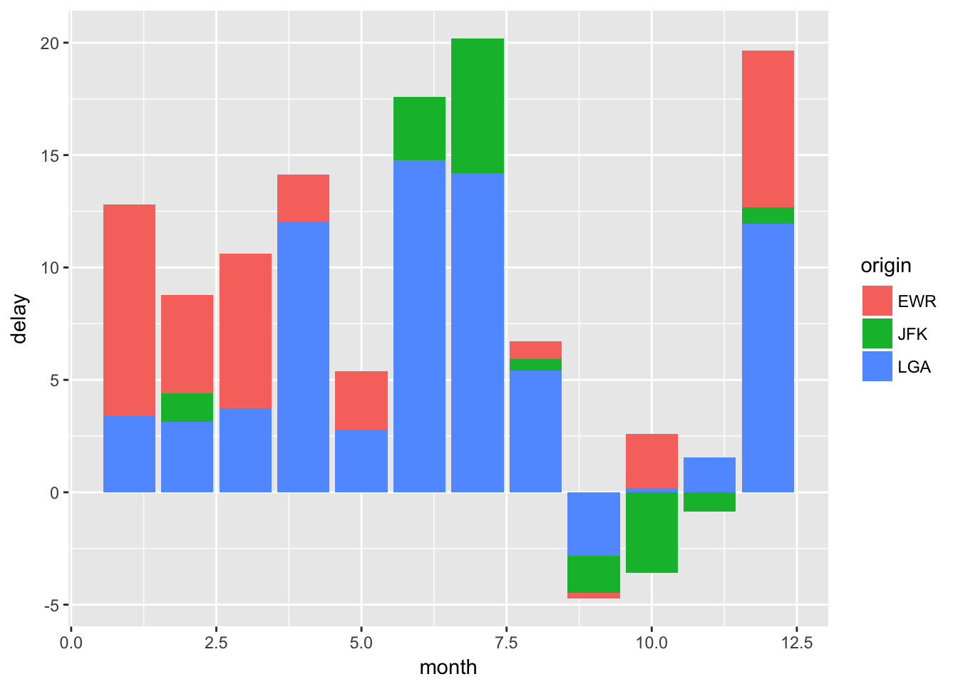
# summertime delays from thunderstorms? winter delays from snow?
# let's look at precipitation
# first lets get the delay by date and origin

# how does weather affect flights?
weather
## # A tibble: 26,130 x 15
## origin year month day hour temp dewp humid wind_dir wind_speed
## <chr> <dbl> <dbl> <int> <int> <dbl> <dbl> <dbl> <dbl> <dbl>
## 1 EWR 2013 1 1 0 37.04 21.92 53.97 230 10.35702
## 2 EWR 2013 1 1 1 37.04 21.92 53.97 230 13.80936
## 3 EWR 2013 1 1 2 37.94 21.92 52.09 230 12.65858
## 4 EWR 2013 1 1 3 37.94 23.00 54.51 230 13.80936
## 5 EWR 2013 1 1 4 37.94 24.08 57.04 240 14.96014
## 6 EWR 2013 1 1 6 39.02 26.06 59.37 270 10.35702
## 7 EWR 2013 1 1 7 39.02 26.96 61.63 250 8.05546
## 8 EWR 2013 1 1 8 39.02 28.04 64.43 240 11.50780
## 9 EWR 2013 1 1 9 39.92 28.04 62.21 250 12.65858
## 10 EWR 2013 1 1 10 39.02 28.04 64.43 260 12.65858
## # ... with 26,120 more rows, and 5 more variables: wind_gust <dbl>,
## # precip <dbl>, pressure <dbl>, visib <dbl>, time_hour <dttm># create new dataset grouped by date and origin adding mean delay
delay_byday_byorigin <- flights %>%
group_by(date, origin) %>%
summarize(delay=mean(arr_delay))
delay_byday_byorigin## # A tibble: 1,095 x 3
## # Groups: date [?]
## date origin delay
## <date> <chr> <dbl>
## 1 2013-01-01 EWR 20.886667
## 2 2013-01-01 JFK 8.088136
## 3 2013-01-01 LGA 7.885593
## 4 2013-01-02 EWR 25.439883
## 5 2013-01-02 JFK 3.268139
## 6 2013-01-02 LGA 7.659259
## 7 2013-01-03 EWR 6.102719
## 8 2013-01-03 JFK 1.766562
## 9 2013-01-03 LGA 10.238095
## 10 2013-01-04 EWR 1.768546
## # ... with 1,085 more rows# Take weather data, group by YMD, summarize mean participation
# remove missing data, add date with lubridate
# join to data created last time
# plot delay by precip coloring by flight's origin, add loess
weather %>% group_by(year, month, day) %>%
summarize(precip = mean(precip)) %>%
na.omit() %>%
mutate(date=ymd(paste(year, month, day, sep="-"))) %>%
inner_join(delay_byday_byorigin, by="date") %>%
ggplot(aes(precip, delay, col=origin)) + geom_point() + geom_smooth()## `geom_smooth()` using method = 'loess' and formula 'y ~ x'## Warning in simpleLoess(y, x, w, span, degree = degree, parametric =
## parametric, : pseudoinverse used at -0.00013056## Warning in simpleLoess(y, x, w, span, degree = degree, parametric =
## parametric, : neighborhood radius 0.00054722## Warning in simpleLoess(y, x, w, span, degree = degree, parametric =
## parametric, : reciprocal condition number 0## Warning in simpleLoess(y, x, w, span, degree = degree, parametric =
## parametric, : There are other near singularities as well. 1.7361e-07## Warning in predLoess(object$y, object$x, newx = if
## (is.null(newdata)) object$x else if (is.data.frame(newdata))
## as.matrix(model.frame(delete.response(terms(object)), : pseudoinverse used
## at -0.00013056## Warning in predLoess(object$y, object$x, newx = if
## (is.null(newdata)) object$x else if (is.data.frame(newdata))
## as.matrix(model.frame(delete.response(terms(object)), : neighborhood radius
## 0.00054722## Warning in predLoess(object$y, object$x, newx = if
## (is.null(newdata)) object$x else if (is.data.frame(newdata))
## as.matrix(model.frame(delete.response(terms(object)), : reciprocal
## condition number 0## Warning in predLoess(object$y, object$x, newx = if
## (is.null(newdata)) object$x else if (is.data.frame(newdata))
## as.matrix(model.frame(delete.response(terms(object)), : There are other
## near singularities as well. 1.7361e-07## Warning in simpleLoess(y, x, w, span, degree = degree, parametric =
## parametric, : at -0.00012361## Warning in simpleLoess(y, x, w, span, degree = degree, parametric =
## parametric, : radius 1.528e-08## Warning in simpleLoess(y, x, w, span, degree = degree, parametric =
## parametric, : all data on boundary of neighborhood. make span bigger## Warning in simpleLoess(y, x, w, span, degree = degree, parametric =
## parametric, : pseudoinverse used at -0.00012361## Warning in simpleLoess(y, x, w, span, degree = degree, parametric =
## parametric, : neighborhood radius 0.00012361## Warning in simpleLoess(y, x, w, span, degree = degree, parametric =
## parametric, : reciprocal condition number 1## Warning in simpleLoess(y, x, w, span, degree = degree, parametric =
## parametric, : zero-width neighborhood. make span bigger## Warning: Computation failed in `stat_smooth()`:
## NA/NaN/Inf in foreign function call (arg 5)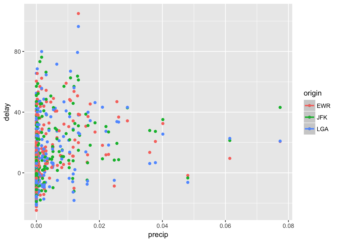
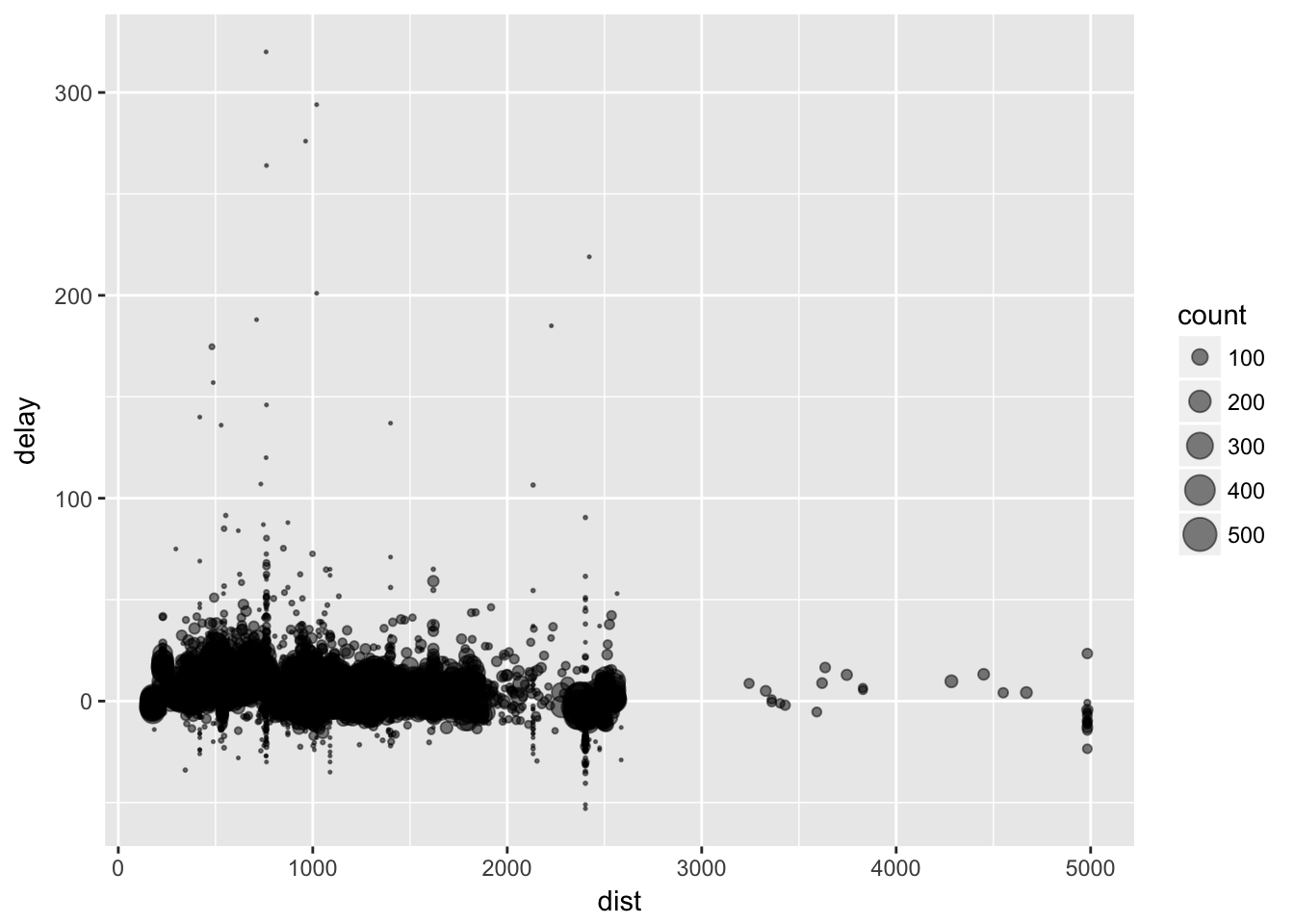
# Is the average delay related to the average distance flown by a plane?
flights %>% group_by(tailnum) %>%
  summarize(dist=mean(distance), delay=mean(arr_delay), count=n()) %>%
  ggplot(aes(dist, delay)) + geom_point(aes(size=count), alpha=1/2) + scale_size_area()