This demonstration of the caret package was given by Mark Lawson, bioinformatician at Hemoshear LLC, Charlottesville VA. The caret package (short for Classification And REgression Training) is a set of functions that streamline the process for creating predictive models. The package contains tools for data splitting, pre-processing, feature selection, model tuning using resampling, and variable importance estimation. Read more about the caret package here.
This demonstration uses the caret package to split data into training and testing sets, and run repeated cross-validation to train random forest and penalized logistic regression models for classifying Fisher’s iris data.
library(caret)## Loading required package: lattice## Loading required package: ggplot2set.seed(42)
# The iris dataset
data(iris)
head(iris)## Sepal.Length Sepal.Width Petal.Length Petal.Width Species
## 1 5.1 3.5 1.4 0.2 setosa
## 2 4.9 3.0 1.4 0.2 setosa
## 3 4.7 3.2 1.3 0.2 setosa
## 4 4.6 3.1 1.5 0.2 setosa
## 5 5.0 3.6 1.4 0.2 setosa
## 6 5.4 3.9 1.7 0.4 setosasummary(iris)## Sepal.Length Sepal.Width Petal.Length Petal.Width
## Min. :4.300 Min. :2.000 Min. :1.000 Min. :0.100
## 1st Qu.:5.100 1st Qu.:2.800 1st Qu.:1.600 1st Qu.:0.300
## Median :5.800 Median :3.000 Median :4.350 Median :1.300
## Mean :5.843 Mean :3.057 Mean :3.758 Mean :1.199
## 3rd Qu.:6.400 3rd Qu.:3.300 3rd Qu.:5.100 3rd Qu.:1.800
## Max. :7.900 Max. :4.400 Max. :6.900 Max. :2.500
## Species
## setosa :50
## versicolor:50
## virginica :50
##
##
## # look at the data
featurePlot(x = iris[, 1:4],
y = iris$Species,
plot = "pairs",
## Add a key at the top
auto.key = list(columns = 3))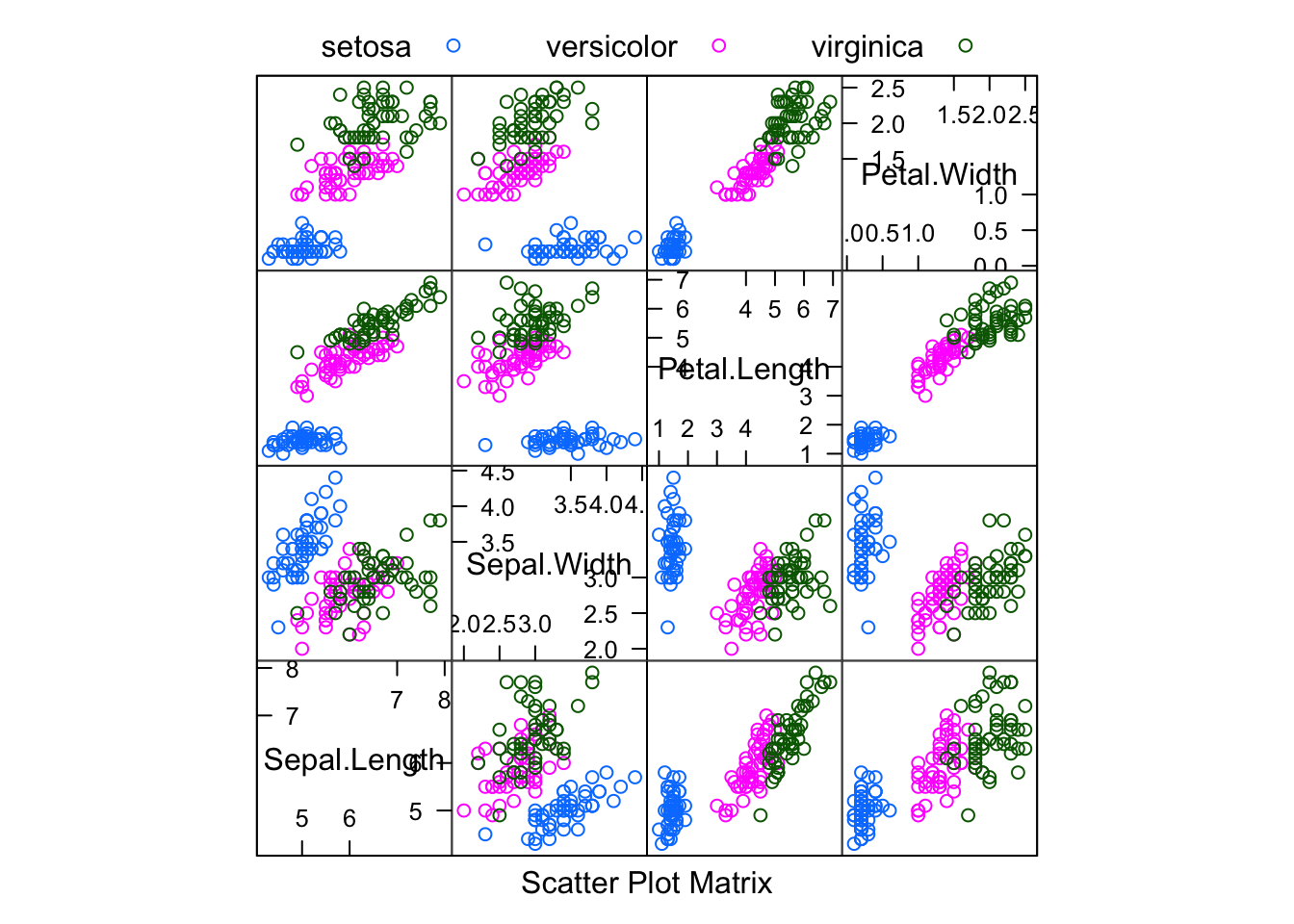
# seperate train and test
trainIndex <- createDataPartition(iris$Species,   # data labels
                                  p = .7,         # percentage used for training
                                  list = FALSE,   # return matrix instead of list
                                  times = 1)      # how many slices?
head(trainIndex)
## Resample1
## [1,] 1
## [2,] 3
## [3,] 4
## [4,] 5
## [5,] 6
## [6,] 7# training data
train_data <- iris[trainIndex,1:4]
train_labels <- iris[trainIndex,5]
# test data
test_data <- iris[-trainIndex,1:4]
test_labels <- iris[-trainIndex,5]
table(train_labels)## train_labels
## setosa versicolor virginica
## 35 35 35table(test_labels)# pre process the data## test_labels
## setosa versicolor virginica
## 15 15 15preprocess_methods <- c("center", "scale")
# determine transformation values
preprocess <- preProcess(train_data,
method=preprocess_methods)
help(preProcess)
# apply transformation values
train_data.pre <- predict(preprocess, train_data)
test_data.pre <- predict(preprocess, test_data)
summary(train_data)## Sepal.Length Sepal.Width Petal.Length Petal.Width
## Min. :4.300 Min. :2.20 Min. :1.100 Min. :0.100
## 1st Qu.:5.200 1st Qu.:2.80 1st Qu.:1.600 1st Qu.:0.300
## Median :5.700 Median :3.00 Median :4.200 Median :1.300
## Mean :5.821 Mean :3.07 Mean :3.748 Mean :1.202
## 3rd Qu.:6.400 3rd Qu.:3.30 3rd Qu.:5.100 3rd Qu.:1.800
## Max. :7.700 Max. :4.40 Max. :6.900 Max. :2.500summary(train_data.pre)## Sepal.Length Sepal.Width Petal.Length Petal.Width
## Min. :-1.9887 Min. :-2.0331 Min. :-1.5096 Min. :-1.4469
## 1st Qu.:-0.8119 1st Qu.:-0.6302 1st Qu.:-1.2245 1st Qu.:-1.1843
## Median :-0.1581 Median :-0.1626 Median : 0.2579 Median : 0.1288
## Mean : 0.0000 Mean : 0.0000 Mean : 0.0000 Mean : 0.0000
## 3rd Qu.: 0.7571 3rd Qu.: 0.5389 3rd Qu.: 0.7711 3rd Qu.: 0.7853
## Max. : 2.4569 Max. : 3.1109 Max. : 1.7974 Max. : 1.7045featurePlot(x = train_data.pre,
y = train_labels,
plot = "pairs",
## Add a key at the top
auto.key = list(columns = 3))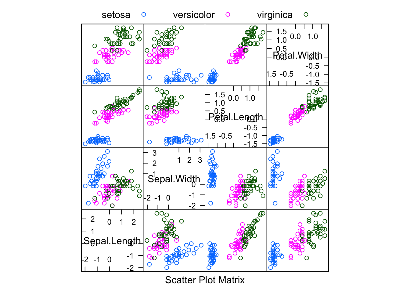
# train the model

# resampling methods / counts
train_control <- trainControl(method = "repeatedcv", # type of resampling
                              number = 10,           # number of folds
                              repeats = 2)           # repeats of whole process

# train a random forest
train_model.rf <- train(x=train_data.pre,      # data
                     y=train_labels,           # labels
                     method="rf",              # classification method
                     trControl=train_control,  # train control
                     metric="Accuracy",        # metric to determine best model
                     tuneLength=3)             # how many tuning parameters to try

train_model.rf
## Random Forest
##
## 105 samples
## 4 predictor
## 3 classes: 'setosa', 'versicolor', 'virginica'
##
## No pre-processing
## Resampling: Cross-Validated (10 fold, repeated 2 times)
## Summary of sample sizes: 94, 94, 94, 95, 94, 95, ...
## Resampling results across tuning parameters:
##
## mtry Accuracy Kappa
## 2 0.9510859 0.9262311
## 3 0.9465404 0.9196066
## 4 0.9465404 0.9196066
##
## Accuracy was used to select the optimal model using the largest value.
## The final value used for the model was mtry = 2.names(train_model.rf)## [1] "method" "modelInfo" "modelType" "results"
## [5] "pred" "bestTune" "call" "dots"
## [9] "metric" "control" "finalModel" "preProcess"
## [13] "trainingData" "resample" "resampledCM" "perfNames"
## [17] "maximize" "yLimits" "times" "levels"# train penalized logistic regression
train_model.plr <- train(x=train_data.pre,
y=train_labels,
method="plr",
trControl=train_control,
metric="Accuracy",
tuneLength=3)
train_model.plr## Penalized Logistic Regression
##
## 105 samples
## 4 predictor
## 3 classes: 'setosa', 'versicolor', 'virginica'
##
## No pre-processing
## Resampling: Cross-Validated (10 fold, repeated 2 times)
## Summary of sample sizes: 94, 94, 95, 95, 95, 94, ...
## Resampling results across tuning parameters:
##
## lambda Accuracy Kappa
## 0e+00 0.6660606 0.4997727
## 1e-04 0.6660606 0.4997727
## 1e-01 0.6660606 0.4997727
##
## Tuning parameter 'cp' was held constant at a value of bic
## Accuracy was used to select the optimal model using the largest value.
## The final values used for the model were lambda = 0.1 and cp = bic.# results of the "best" model
train_model.rf$finalModel##
## Call:
## randomForest(x = x, y = y, mtry = param$mtry)
## Type of random forest: classification
## Number of trees: 500
## No. of variables tried at each split: 2
##
## OOB estimate of error rate: 4.76%
## Confusion matrix:
## setosa versicolor virginica class.error
## setosa 35 0 0 0.00000000
## versicolor 0 33 2 0.05714286
## virginica 0 3 32 0.08571429train_model.plr$finalModel##
## Call:
## stepPlr::plr(x = x, y = y, weights = if (!is.null(wts)) wts else rep(1,
## length(y)), lambda = param$lambda, cp = as.character(param$cp))
##
## Coefficients:
## Intercept Sepal.Length Sepal.Width Petal.Length Petal.Width
## -3.24506 -1.32064 1.45670 -2.41441 -2.13541
##
## Null deviance: 133.67 on 104 degrees of freedom
## Residual deviance: 1.42 on 102.18 degrees of freedom
## Score: deviance + 4.7 * df = 14.53# dive into the final model
class(train_model.rf$finalModel)## [1] "randomForest"names(train_model.rf$finalModel)## [1] "call" "type" "predicted"
## [4] "err.rate" "confusion" "votes"
## [7] "oob.times" "classes" "importance"
## [10] "importanceSD" "localImportance" "proximity"
## [13] "ntree" "mtry" "forest"
## [16] "y" "test" "inbag"
## [19] "xNames" "problemType" "tuneValue"
## [22] "obsLevels" "param"plot(train_model.rf$finalModel)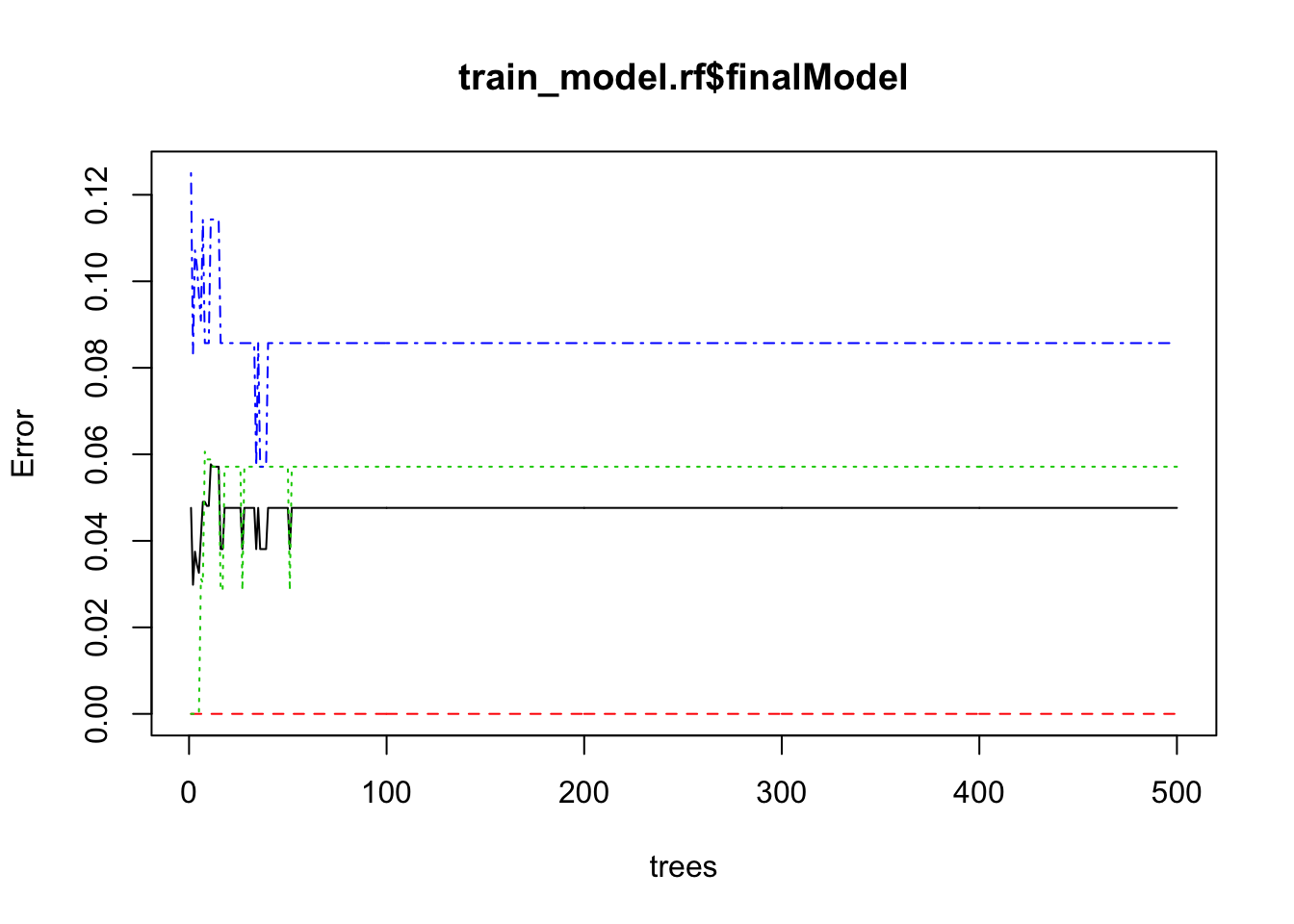
class(train_model.plr$finalModel)## [1] "plr"names(train_model.plr$finalModel)## [1] "coefficients" "covariance" "deviance"
## [4] "null.deviance" "df" "score"
## [7] "nobs" "cp" "fitted.values"
## [10] "linear.predictors" "level" "call"
## [13] "xNames" "problemType" "tuneValue"
## [16] "obsLevels" "param"# apply to test data
results.rf <- predict(train_model.rf, test_data.pre)
results.plr <- predict(train_model.plr, test_data.pre)
# side by side results
View(data.frame(test_labels,
results.rf,
results.plr))
# stats for the results
confusionMatrix(data=results.rf,
reference=test_labels)## Confusion Matrix and Statistics
##
## Reference
## Prediction setosa versicolor virginica
## setosa 15 0 0
## versicolor 0 13 1
## virginica 0 2 14
##
## Overall Statistics
##
## Accuracy : 0.9333
## 95% CI : (0.8173, 0.986)
## No Information Rate : 0.3333
## P-Value [Acc > NIR] : < 2.2e-16
##
## Kappa : 0.9
## Mcnemar's Test P-Value : NA
##
## Statistics by Class:
##
## Class: setosa Class: versicolor Class: virginica
## Sensitivity 1.0000 0.8667 0.9333
## Specificity 1.0000 0.9667 0.9333
## Pos Pred Value 1.0000 0.9286 0.8750
## Neg Pred Value 1.0000 0.9355 0.9655
## Prevalence 0.3333 0.3333 0.3333
## Detection Rate 0.3333 0.2889 0.3111
## Detection Prevalence 0.3333 0.3111 0.3556
## Balanced Accuracy 1.0000 0.9167 0.9333confusionMatrix(data=results.plr,
reference=test_labels)## Confusion Matrix and Statistics
##
## Reference
## Prediction setosa versicolor virginica
## setosa 15 0 0
## versicolor 0 15 15
## virginica 0 0 0
##
## Overall Statistics
##
## Accuracy : 0.6667
## 95% CI : (0.5105, 0.8)
## No Information Rate : 0.3333
## P-Value [Acc > NIR] : 5.001e-06
##
## Kappa : 0.5
## Mcnemar's Test P-Value : NA
##
## Statistics by Class:
##
## Class: setosa Class: versicolor Class: virginica
## Sensitivity 1.0000 1.0000 0.0000
## Specificity 1.0000 0.5000 1.0000
## Pos Pred Value 1.0000 0.5000 NaN
## Neg Pred Value 1.0000 1.0000 0.6667
## Prevalence 0.3333 0.3333 0.3333
## Detection Rate 0.3333 0.3333 0.0000
## Detection Prevalence 0.3333 0.6667 0.0000
## Balanced Accuracy 1.0000 0.7500 0.5000# variable importance
varImp(train_model.rf)## rf variable importance
##
## Overall
## Petal.Width 100.00
## Petal.Length 89.18
## Sepal.Length 13.90
## Sepal.Width 0.00train_model.rf$finalModel$importance## MeanDecreaseGini
## Sepal.Length 6.457729
## Sepal.Width 2.358824
## Petal.Length 28.651485
## Petal.Width 31.840657